This is an old revision of the document!
Table of Contents
Commit 2018-07-03
In this commit, the Metafor component of the new coupling procedure with Metalub is added. First, the version and folder structure is explained (which Metalub version is coherent with the current Metafor version? what versions did Carretta use in his coupling procedure?). Then, the details of the Metafor model are described: geometry, mesh, material, boundary conditions, data extraction, regression tests.
Versions and folder structure
This commit is related to the commits 1454 to 1456 of Metalub. For optimal conherence between Metalub and Metafor, commit 1456 of Metalub should be checked out with this version of Metafor, if the coupling procedure is used.
The Metafor component of Carretta's version of the coupling procedure was kept in Metafor, although it was deleted in Metalub due to a significant code architecture dependence, i.e. it was very complex to add another co-existant coupling component in Metalub without deleting Carretta's version, which had in any case significant drawbacks (see commit 1454 of Metalub). The Carretta's old coupling procedure can be used by checking out the commits 3071 and 1376 of Metafor and Metalub, respectively.
Concerning the folder structure, the Metafor component of the new coupling procedure with Metalub can be found in the folder aspCrushing/boemer. The folder tests contains two folders bcDry and bcLub, which contain the boundary conditions of the two new Metafor test cases mtfrTest5B4DryLinear.py and mtfrTest5B4LubLinear.py. These test cases are based on the experimental test 5B with a rolling speed of about 200 m/min at Maizière-lès-Metz in 2014, once without lubricant, once with lubricant (see Boemer's report maiziere2014.pdf, which will be a part of his thesis). The boundary condition files were copied from the first Metafor computation of the coupling test cases in Metalub, see folders cplMetafor/tests/dry/jortnerRoll and cplMetafor/tests/lub/rigidCircularRoll of Metalub. The folder tools contains the different scripts, which are necessary to build a general asperity flattening FE model. The main script is flattening.py, which uses the file geoLinear.py to build the geometry and the mesh, and the file extractors.py to define some custom extractors.
Geometry
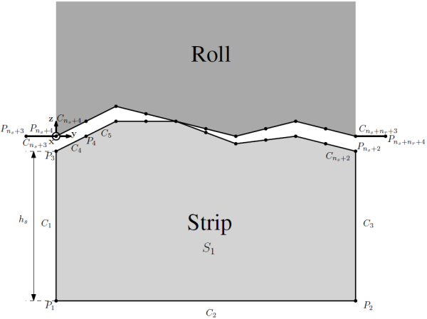
The finite element model is constructed in a plane, which is normal to the rolling direction. It consists of a rigid set of line segments, representing the roll, with an arbitrary profile that is fixed in space and a portion of the strip. The upper edge of the strip has an arbitrary profile, too, while its other edges are straight. The following figure illustrates the geometry with its points $P_{i}$, curves $C_{i}$ and surface $S_{1}$. The points $P_{3}$ and $P_{n_{s}+2}$ should have the same $y$-coordinates than $P_{n_{s}+4}$ and $P_{n_{s}+n_{r}+3}$, respectively, where $n_{s}$ and $n_{r}$ are the number of points of the strip and the roll profile, respectively. It is important to notice that a different system of coordinates is used in the Metafor data set than in the following figure. In Metafor, the rolling direction is $\mathbf{z}$ and the vertical direction $\mathbf{y}$; this allows to define the model in the $xy$-plane in Metafor. The profiles of the roll and the strip could initially not be in contact unlike what is shown in the following figure. The Python input script translates them accordingly in this case. Besides the profiles of the roll and the strip, the geometry depends on the definition of $h_{s}$, the thickness of the strip substrate portion. The points $P_{n_{s}+3}$ and $P_{n_{s}+n_{r}+3}$ (and the respective curves) were added to extend the contact tool.
It is important to notice that these points should not be taken into account in the computation of the mean line position, nor that of the relative contact area.
The upper edge of the strip and the lower edge of the roll are represented by linear segments. This could lead to contact detection problems depending on the particular geometry of the roll's edge. Currently, the profiles (without extensions for the roll) are, however, represented by single line segments, for which contact detection is relatively trivial. If problems arise for more complex geometries, the lines segments could be replaced by splines or MultiProjWires.
Mesh
The mesh of the strip portion $S_{1}$ is a quadrilateral mesh parameterized by $n_{x}$, $n_{y}$ and $r_{ny}$, the number of elements along $\mathbf{x}$, the number of elements along $\mathbf{y}$ and the ratio between the smallest and the largest side lengths of the elements along $\mathbf{y}$. The ratio $r_{ny}$ is chosen in such a way that the aspect ratio of the elements of the top strip layer is 1, since there might be located the most significant field gradients.
Material
The material law is the same than in the Metalub computation. This is an assumption since the surface layer of the strip might have different properties than the underlying bulk material.
Boundary conditions
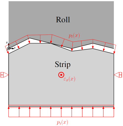
The following figure illustrates the boundary conditions of the FE model:
- The edge which represents the roll profile is fixed in space.
- The lateral edges of the strip can move only along the vertical axis.
- The displacements of all nodes on the lower edge of the strip portion is identical along $\mathbf{z}$.
- The evolution of the interface pressure $p_{i}$ is applied to the lower edge of the strip, which pushes it against the contact tool.
- The evolution of the lubricant pressure $p_{l}$ is applied to the upper edge of the strip, which pushes it downwards.
- The evolution of the out-of-plane elongation $\epsilon_{x}$ is applied to the strip portion.
The evolutions of $p_{i}$, $p_{l}$ and $\epsilon_{x}$ along the roll bite can be transformed into evolutions along time, simply by assuming that $x = t$, which is possible since the material model is independent of time. The velocities in the model should also be sufficiently small to have negligible inertial effects.
Data extraction
During the evolution of the interface pressure and the strip elongation, the relative contact area $A$ and the distance between updated mean lines $h_{t}$ is computed.
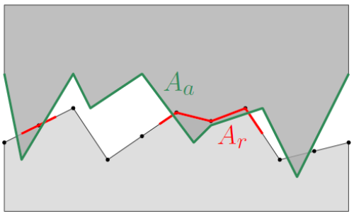
Different ways of computing the relative contact area are possible. Carretta computed the contact area as illustrated in the following figure, which is coherent with the contact force computation. More precisely, if a node of the strip is suddenly in contact with the roll, the contact area increases by the contact area associated to this node, which is equal to the sum of the half-lengths of the incident segments of the node multiplied by the out-of-plane thickness. To obtain the relative contact area $A = A_{r}/A_{a}$, the total contact area $A_{r}$ is divided by the total length of the strip profile and the out-of-plane thickness, which are assumed to be an approximation of the apparent contact area $A_{a}$. Depending on the shape of the strip profile, different relative contact areas $A$ can be obtained for the same contact area $A_{r}$. This is why a different way of computing the relative contact area was introduced.
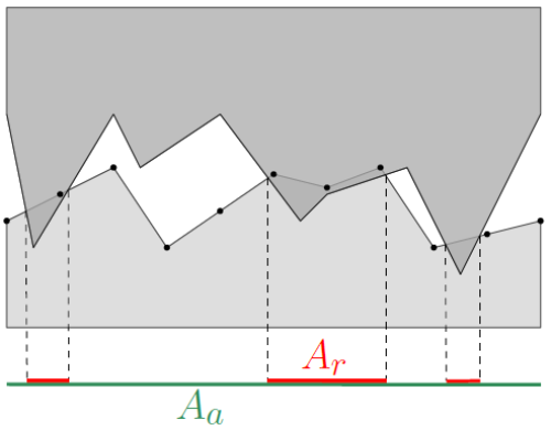
In this coupling procedure, the approach illustrated in the following figure was not only implemented to obtain a more objective measure of the relative contact area, but also to have a smoother evolution of the relative contact area, i.e. previously, the contact area increased suddenly by the nodal contact area, when the respective node of the strip got in contact with the roll. Although this smoothness intuitively seems to lead to better results, this has still to be tested.
Regression tests
As mentionned earlier, the following tests were added:
- aspCrushing.boemer.tests.mtfrTest5B4DryLinear.py
- aspCrushing.boemer.tests.mtfrTest5B4LubLinear.py
To check whether these tests do not change from one version of Metafor to the next, only one specific value per test is currently added to the TSC. It is the realtive contact area $A$ at -5.8 mm in the roll bite.


