This is an old revision of the document!
Table of Contents
How to build my own FE model?
Introduction
Before reading this page, the document Python in a nutshell must be read and understood. In other words, you must be able to use a Python interpreter in a basic way.
In the following document are described, line after line, the steps leading to the development of a input file where a cylindrical die will crush a block of material in plane strain. Here is a preview of the final deformation.
<html>
<embed width=“320” height=“240” src=“http://metafor.ltas.ulg.ac.be/oldsite/flv/flvplayer.swf?file=http://metafor.ltas.ulg.ac.be/oldsite/flv/tuto.flv” quality=“high” type=“application/x-shockwave-flash” />
</html>
Since Metafor is continuously improved and modified, the syntax of some commands may have slightly changed since the writing of this documentation. However, this input file is part of the test battery, so a working file corresponding to your version of Metafor can be found in apps\tutorials\tutorial1.py.
Input-file Description
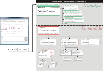
A Metafor input file is a Python module which defines an object called Metafor. This main object will be retrieved and used by the GUI once the user presses the blue PLAY button. The image below shows a schematic organization of a module and the hierarchical structure of the various objects that will be involved in the test case.
To sum up, one input file = one (or several) Python files = one Metafor object.
Heading
The module usually begins with some Python comments (preceded by “ # ”) .
# -*- coding: latin-1; -*-
# $Id$
#
# Tutorial
The line “coding” is required if we want to use accented characters in python. The “SVN tag” $Id$ (optional) allows us to know the version of this file.
from wrap import *
import math
The first line imports the Python/C++ interface of Metafor (called wrap) in the current namespace, so that all compiled C++ objects of Metafor are available in Python.
The math module is also imported, in this case, to use the functions sine and cosine later.
metafor = Metafor()
domain = metafor.getDomain()
The main object of the module ) is now created as an instance of the Metafor class. This command Metafor() creates an object Metafor, from which we can extract a Domain. The domain is a container (see References). It contains all objects that are required by the model (geometry, elements, nodes, fixations and other boundary conditions, materials, …).
The analysis will then handle data from this domain to, for example, integrate temporally over its evolution equations.
The only function of the module that Metafor requires to work properly is the function getMetafor() which must return the analysis, metafor. This function is automatically called during the initialization when using the command meta.
def getMetafor(p={}): return metafor
The parameter p is an optional dictionary used for parametric studies.
Parameters
Parameters should always be used instead of numbers, to easily modify the model. Indeed, one Finite Element simulation alone hardly has any meaning, the solution must be checked by varying numerical parameters. For this reason, all parameters are gathered in the beginning of the module, to modify them easily.
Lx = 1.0  # length X
Ly = 1.0  # length Y
n1 = 10   # nb of elems on X
n2 = 10   # nb of elems on Y
Four parameters are defined: the length and width of the rectangle to mesh, and the number of mesh elements in the two directions.
Geometry
Now, a “user” geometry is defined (in opposition to a “mesh” geometry, which will be automatically generated when meshing the part). To do so, a Python reference pointing towards the “geometry” object (type Geometry) is retrieved from the just-created domain.
geometry = domain.getGeometry()
geometry.setDimPlaneStrain(1.0)
The first line retrieves the reference from the domain. The second line sets the type of geometry. Here, plane strain is chosen, but axisymmetric or 3D are also possible (see Structure of a Metafor module).
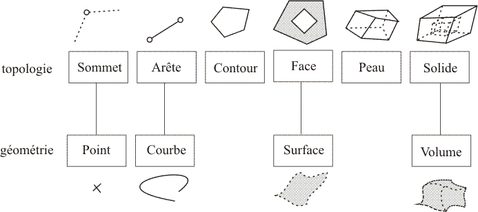
Defining a geometry always follows the same pattern (see figure above). In Metafor, a simplified Boundary Representation (B-REP) is used, where each entity is defined as a set of lower level entities:
- The
Volumeobject, the 3D entity of highest level, consists of one or severalSkins: one external one and a set of holes. - A
Skinconsists of an ordered set ofSides.
This is called a simplified B-REP (see figure below) because geometric and topological concepts are mixed for curves and points. In a traditional B-REP, a curve would be defined as an edge consisting of two vertices, to which a geometry is associated.
To each geometric entity is associated a Set. Thus, the objects Points are gathered in a PointSet, the objects Curves in a CurveSet… All these sets are included in the object Geometry. To access them, a function get*() is used (getPointSet(), …).
Geometric objects can be defined in two ways, depending on their size and complexity :
- Bigger objects which require more arguments, like curves, are defined using a temporary object, which is filled and copied. For example, a curve is created by first defining a line (see below).
In this example, Points are defined with the first method, as the function named “define”. The first argument is a user number, which must be strictly positive and different for each entity in a common set. The next three arguments are the spatial coordinates $x, y \mbox{ and } z$. Since the geometry was set to plane strain, the default plane $z=0$ is considered and only $x$ and $y$ are given.
pointset = geometry.getPointSet()
pointset.define(1,  0,   0)
pointset.define(2,  Lx,  0)
pointset.define(3,  Lx, Ly)
pointset.define(4,  0,  Ly)
pointset.define(5,  2*Lx,  Ly+2*Lx)
pointset.define(6,  2*Lx*math.cos(math.pi/4),
                  Ly+2*Lx-2*Lx*math.sin(math.pi/4))
pointset.define(7, -2*Lx, Ly+2*Lx)
Next, the curves are defined:
curveset = geometry.getCurveSet()
curveset.add(Line(1, pointset(1), pointset(2)))
curveset.add(Line(2, pointset(2), pointset(3)))
curveset.add(Line(3, pointset(3), pointset(4)))
curveset.add(Line(4, pointset(4), pointset(1)))
curveset.add(Arc(5, pointset(7), pointset(6), pointset(5)))
The first line retrieves a reference pointing towards the set of all curves, named CurveSet. Curves can be of different types (lines, arcs, …) and sometimes quite complex (Nurbs), therefore the second method is used: creating the object, then adding it to the set. The function Line requires three argument, a user number and the two end points, when the function Arc requires three points.
The arc is defined to model a contact matrix. Therefore, its orientation matters and must be defined with “area on the left”. This means that, if the arc is followed in the way given by the succession of its points, the die will be on the left hand side.
After the curves come the wires:
wireset = geometry.getWireSet()
wireset.add(Wire(1, [curveset(1), curveset(2), curveset(3), curveset(4)]))
Wires are defined in the same way as curves. Two arguments are required, the user number and the Python tuple, [curveset(1), curveset(2), curveset(3), curveset(4)], which contains the curves.
Finally, the highest order element for a 2D case, the side, is also defined with the second method (create object then add it to the container WireSet).
sideset = geometry.getSideSet()
sideset.add(Side(1,[wireset(1)]))
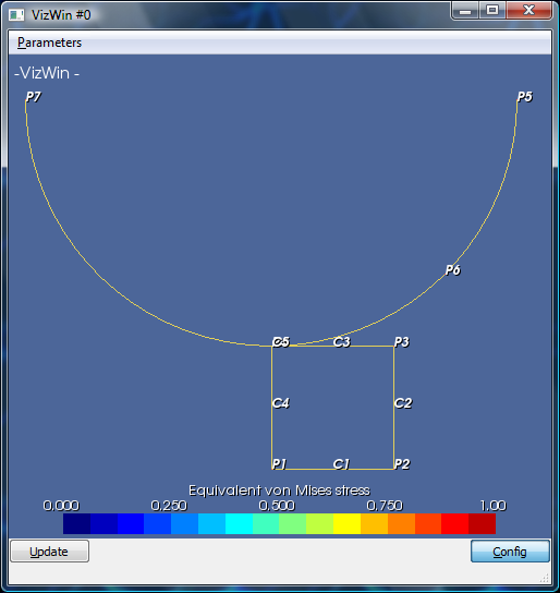
At this point, the whole geometry is defined, so it is recommended to check whether this was done properly. To do so, viewing tools coming from the wrap module can be used (this module was imported at the very beginning), with the command lines:
if 1:
    win = VizWin()
    win.add(pointset)
    win.add(curveset)
    win.open()
With these lines, a new VizWin object (graphical window) named win is created. The points and curves are added to this object. The function open() finally opens the window.
These lines are included in a “if block”, easy to activate and deactivate by replacing the 1 by a 0 and vice versa.
To view the geometry, Metafor must be run and the module loaded with the GUI or imported with the command
import apps.qs.tutorial
Another way to check the geometry is with the function print. For instance, print geometry gives a summary of the contents of the container Geometry.
Mesh
Now, the model must be meshed. This could also be done later one, because the boundary conditions are defined based on the user geometry and not on the mesh itself. Indeed, the user will not have to handle neither mesh, elements nor nodes. It is always much better to define boundary conditions based on the user geometry, since the mesh is the first parameter that is usually changed to verify the solution. Therefore, if some conditions are defined based on nodes number, they must be changed every time the mesh is refined. All of this to say that meshing the part could be done later on.
SimpleMesher1D(curveset(1)).execute(n1)
SimpleMesher1D(curveset(2)).execute(n2)
SimpleMesher1D(curveset(3)).execute(n1)
SimpleMesher1D(curveset(4)).execute(n2)
TransfiniteMesher2D(sideset(1)).execute(True)
As could be seen above, an object in a set is accessed with the use of parentheses (there is one exception regarding the list of materials, and old Oofelie object still requiring brackets). For example, a reference towards curve 2 is retrieved with the line curveset(2).
The meshers (1D Mesher, 2D Mesher) are linked to the entity that must be meshed and executed with the command execute(). For face 1, the integrated mesher TIM (Transfinite Interpolation Method), suitable for quadrangles where two opposite edges have the same numbers of elements, is used.
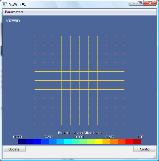
As for the geometry, it is recommended to visually check whether the piece was meshed properly by opening a VizWin window with the following lines :
if 1:
  win = VizWin()
  win.add(geo.getMesh().getPointSet())
  win.add(geo.getMesh().getCurveSet())
  win.open()
  raw_input()
The geometry to display is called “mesh” (the mesh geometry also contains neighboring relations).
It is also possible to use the function print to display a list of all mesh elements, edges and vertices.
Defining volume elements
Now that the geometry is defined, physical properties must be assigned to the domain, by associating (Finite Elements) to the mesh. Here, 2D-volume elements will be used.
Material
First, the volume behavior of the block which is to be crushed is defined. This is done by defining a material. The set of all materials can be found in the domain.
materialset = domain.getMaterialSet()
materialset.define (1, EvpIsoHHypoMaterial)
materialset(1).put(MASS_DENSITY,     8.93e-9)
materialset(1).put(ELASTIC_MODULUS, 200000.0)
materialset(1).put(POISSON_RATIO,        0.3)
materialset(1).put(YIELD_NUM,             1)
A law to model hardening is also required. This law must be defined in the set MaterialLawSet, also found in the domain
lawset = domain.getMaterialLawSet()
lawset1 = lawset.define (1, LinearIsotropicHardening)
lawset1.put(IH_SIGEL, 400.0)
lawset1.put(IH_H,    1000.0)
When looking at the commands above, defining a material is done by calling the MaterialSet function named define(), with the material number and type as arguments. Here, the elastic plastic material named EvpIsoHHypoMaterial is chosen.
A reference point towards the newly created object can be retrieved with the parenthesis operator (materialset1 = materialset(1)), but this reference is also supplied by the function define() (materialset1 = materialset.define (1, EvpIsoHHypoMaterial)).
After defining the type of material, the material function put() is used to define the required parameters, such as Young Modulus, density, …
With this function, a hardening law was also associated to the material using the YIELD_NUM code. This law is defined in the same way as a material, in the set named MaterialLawSet (retrieving a reference from the domain, defining the law, then assigning its parameters). Here, a linear isotropic hardening is assumed, so the required parameters are the yield stress (IH_SIGEL) and the hardening coefficient (IH_H). Each law and material have their own codes.
Element Properties
Before defining Finite Elements, an object called ElementProperties must be defined. This ElementProperties will link the newly defined materials to these Finite Elements.
prp1 = ElementProperties(Volume2DElement)
prp1.put(MATERIAL, 1)
prp1.put(CAUCHYMECHVOLINTMETH, VES_CMVIM_SRIPR)
It is when defining an Element Properties that the desired type of Finite Element is specified. Here, the type Volume2DElement is chosen, but other possibilities exist. For example, the thermomechanical TmVolume2DElement could also be used if heat transfer was significant.
It is also at this point that the use of the selective SRI integration with pressure report is set, to avoid locking.
Element Generator - FieldApplicator
Finally, an element generator is used to apply the newly defined Element Properties to the meshed geometry. In Metafor, these objects are called interactions“. The generator in charge of volume elements is the FieldApplicator
app = FieldApplicator(1)
app.push(sideset(1))
app.addProperty(prp1)
interactionset = domain.getInteractionSet()
interactionset.add(app)
The FieldApplicator has a user number, and is defined in the set InteractionSet, which can also be found in the domain.
Then, this element must be applied to a part of the meshed geometry, with the command push() (here to sideset(1)). Generating Finite Elements is always associated to a geometric entity, not to the mesh itself. Linking the mesh to the Finite Elements is internally done by Metafor.
Afterwards, the Element Properties is added to the interaction, with the command addProperty().
Before going further, a ”print interactionset“ should be run to display all interactions (see Volume interaction).
Boundary Conditions
Fixed end
Now, the boundary conditions are considered. The set which handles all boundary conditions commands is called the LoadingSet.
The X component of ligne 4 and the Y component of line 1 must be fixed, by symmetry.
loadingset = domain.getLoadingSet()
loadingset.define(curveset(4), Field1D(TX,RE))
loadingset.define(curveset(1), Field1D(TY,RE))
In these lines, the object Field1D passed in argument is a code which designates the degree of freedom which must be fixed. Here, TX,RE stands for “Translation along X”, RElative value, which is the displacement along X.
Loadings (non-zero displacement, static load, ...)
In this test case, the motion of the die over time must be described. To do so, a function d=f(t) is defined, for example with the class called PieceWiseLinearFunction :
fct = PieceWiseLinearFunction()
fct.setData(0.0, 0.0)
fct.setData(1.0, 1.0)
This non-zero displacement is defined with the LoadingSet :
loadingset.define(curveset(5), Field1D(TY,RE), -0.4, fct)
Setting fixed ends or displacements is done is the same way as the definition of points in the geometry, with the single define() command. For the non-zero displacement of the die, the geometric entity curveset(5) is first given, then the direction TY,RE (= displacement along Y), the amplitude -0.4 and finally the temporal evolution, with the reference to the function fct. This means that the movement will be described with d(t) = -0.4 * fct(t) = -0.4 * t
Contact
Contact is managed by contact elements. A new set of elements must be defined, in the same way as volume elements : first with a contact material, then an ElementProperties, and finally with an element generator (interaction).
The material chosen is called StickingContactMaterial (second material put in MaterialSet) :
materialset.define(2, StickingContactMaterial)
materialset(2).put(PROF_CONT,    0.05)
materialset(2).put(PEN_TANGENT,  10000)
materialset(2).put(PEN_NORMALE, 10000)
Then, the ElementProperties Contact2DElement links this material to the finite elements to be defined, and set the type of element to generate.
prp2 = ElementProperties(Contact2DElement)
prp2.put (MATERIAL, 2)
Finally, the element generator. Several can be chosen, depending on how contact is modeled. Here, contact is between a rigid entity, the die, and a deformable entity, the meshed solid. The corresponding generator is called RdContactinteraction, where Rd stands for Rigid-Defo :
ci = RdContactInteraction(2)
ci.setTool(curveset(5))
ci.push(curveset(3))
ci.addProperty(prp2)
interactionset.add(ci)
The deformable entity is specified with the command push(), the rigid one with setTool().
It should be noted that the contact interaction number must be different that the FieldApplicator number defined earlier, since both objects are included in the same set InteractionSet.
Temporal Integration
The description of this model is now over. What is left to consider is the way the Metafor analysis, in charge of running the simulation, will integrate the equations temporally.
Many options are available, however the simplest one is chosen here, which is a quasi-static integration (where the inertia is neglected). What remains to define is the temporal interval on which the simulation will be run, and the way the results will be saved (see Managing Time Steps).
tsm = metafor.getTimeStepManager()
tsm.setInitialTime(0.0, 0.01)
tsm.setNextTime(1.0, 1, 1.0)
The TimeStepManager of Metafor is used to specify the relevant parameters.
First, the initial time, $t=0$ and the initial time step, $d_t = 0.01 s$ are set using the command setInitialTime. Afterwards, the time step will be adjusted automatically if needed.
Then, the command setNextTime() is used to specify the next steps of the simulation (here, only one step corresponding to the final time $t = 1 s$ is considered), the number of times data must be saved on disk (here, only one in addition to the initial configuration, so two saving points), and the maximal time step which can be used during this interval ($d_t = 1.0 s$).
mim = metafor.getMechanicalIterationManager()
mim.setMaxNbOfIterations(7)
mim.setResidualTolerance(1.0e-4)
Afterwards, the MechanicalIterationManager is considered (see Managing N.-R. Iterations). This object sets the parameters of Newton-Raphson algorithm, used to solve the equilibrium equations. Here, a maximum of 7 mechanical iterations is set, with the default tolerance of 1.0e-4.
Curves Extraction
It is also possible to save some result curves, which are defined as the temporal evolution of a variable on a given geometric entity.
valuesmanager = metafor.getValuesManager()
valuesmanager.add(1, MiscValueExtractor(metafor,EXT_T),'time')
valuesmanager.add(2, DbValueExtractor(curveset(1), Field1D(TY,GF2)), SumOperator(), 'force')
The first line fetches the ValuesManager, in charge of handling the result curves, from the analysis Metafor.
The second line defines the first curve, which will save the time value at each time step.
The third line defines a second result curve which extracts the value Field1D(TY,GF2) (external forces), at each node of the geometric curve 1, then sums all these values and writes it under the name force.
These curves can be viewed in real time in VizWin, see Viewing curves in real time.
Running the simulation
First, the test case must be loaded using the command load('apps.qs.tutorial'), if the module is named ”tutorial.py“ and is located in the folder apps/qs.
Then, the integration is started with the command meta().
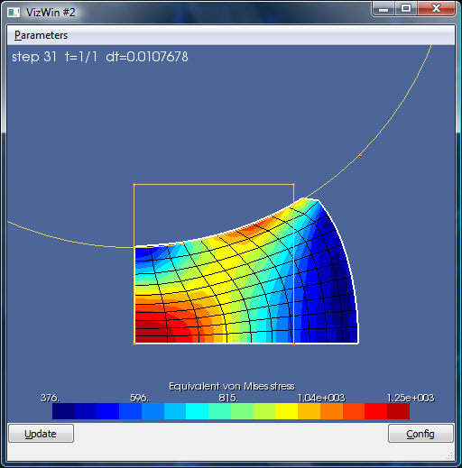
If everything was done properly, this famous figure is obtained
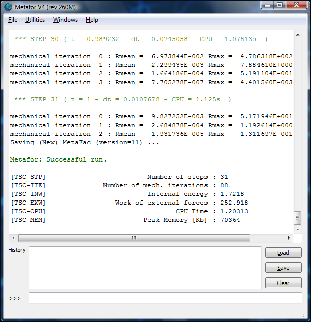
At the same time, the python window indicates the temporal integration was successful.
Viewing Results
Loading Saved Configurations
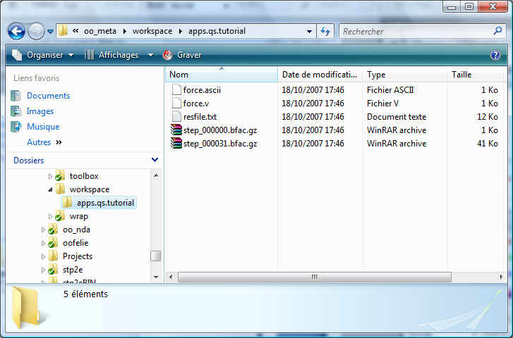
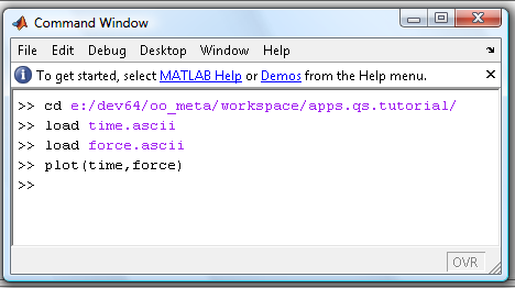
Using VizWin and real time viewing, it is possible to follow the temporal integration. During this integration, some saving files (.bfac.gz) are created and may be read again once the integration is completed.
This was explained in details in How to run an existing test?.
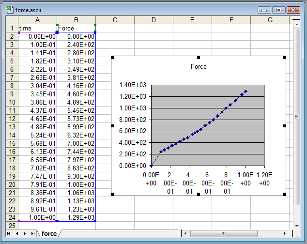
Viewing Curves Using Excel
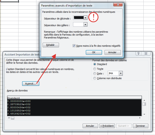
Run Excel, and load the desired .ascii files (time.ascii et force.ascii in this example). Use the filter “All files *.*”.
A box opens to configure the importation. At this point, it is important to check that the point ”.“ is set as decimal separator (see figure below).
Once both files are imported, the two data columns must be placed on a single sheet, and a 2D plot must be defined when selecting the data.
The result is shown on the following figure :

