Table of Contents
Commit 2017-12-20
In this commit, the asperity crushing simulations in the generalized plane strain state created by Carretta for the Metalub/Metafor coupling were simplified as much as possible and corrected where necessary. The scripts of these simulations can be found in:
oo_meta\aspCrushing\tests\twoDHalf;oo_meta\aspCrushing\tools\twoDHalf.
The first directory contains 6 test cases and the input data of these test cases:
splineDry.py: spline shaped asperity crushing without lubricant;splineLub.py: spline shaped asperity crushing with lubricant;triangle1Dry.py: single triangular shaped asperity crushing without lubricant;triangle1Lub.py: single triangular shaped asperity crushing with lubricant;triangle2Dry.py: double triangular shaped asperity crushing without lubricant;triangle2Lub.py: double triangular shaped asperity crushing with lubricant;profilBertrandieBattery.ascii: a real asperity profile used in splineDry.py and in splineLub.py;bc: directory containing Metalub results, which are used in the boundary conditions of all test cases. See Metalub for more detailed explanations, especially the reference document created by Boemer.
The second directory contains parameterized scripts that are used to build the simulation of the 6 test cases:
aspCrush.py: script that builds most of the simulation. Among other things, it uses the following scripts to build the geometry, mesh, …, and to extract the required data of the results;geoTriangle1.py,geoTriangle2.pyandgeoSpline.py: scripts that build the geometry, mesh, ALE rezoners and that compute the vertical position of the mean line of the roll asperity;aspExtr.py: script that defines the extractors used inaspCrush.py;Vector.py,Profil.pyandevolutionFunction.py: scripts with basic operations to keep the commands inaspCrush.pyas short and meaningful as possible.
Notice that the rolling direction in this model is aligned with the axis $\mathbf{z}$, while the vertical axis is $\mathbf{y}$ since plane strain simulations are usually represented in the $xy$-plane. In Metalub, the rolling direction is $\mathbf{x}$ and the vertical direction is $\mathbf{y}$ since cold rolling was first modeled in 2D. To extend the model to 3D, even another but more general choice was made in the reference document by Boemer, i.e. the rolling direction is $\mathbf{x}$ and the vertical axis is $\mathbf{z}$.
CMakeLists.txt
The following line was added in the IF(MSVC) of the main CMakeLists.txt file to enable parallel compilation even without IncrediBuild:
SET(CMAKE_CXX_FLAGS "${CMAKE_CXX_FLAGS} /MP")
Geometries, Meshes and ALE Rezoners
The asperity crushing simulations were created in 2D for computation time reasons. The rolling direction is aligned with the $\mathbf{z}$-axis in these simulations and the asperity profile is represented in the orthogonal plane to the rolling direction. This orientation was chosen due to its similarity to the cold rolling scenario with grinded rolls. In fact, after grinding, the rolls have an asperity profile that changes mainly along the axial direction and which has a more important amplitude than the asperity profile of the strip. Due to the greater hardness of the roll with respect to the strip, one can therefore say, that asperity crushing is best simulated in an orthogonal plane to the rolling direction.
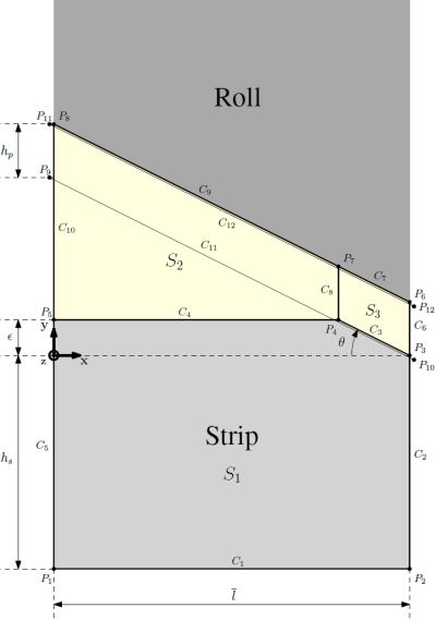
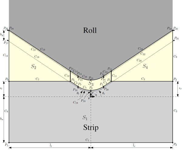
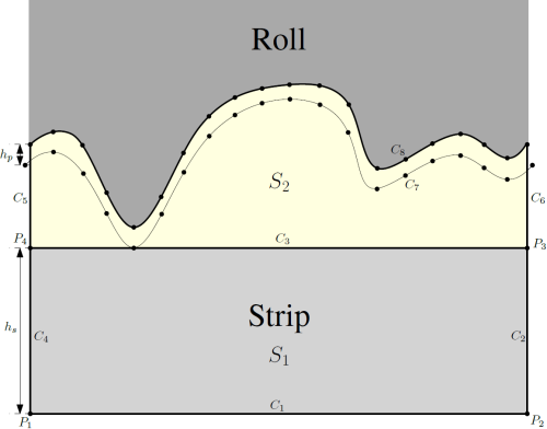
For reasons of clarity, the following figures were created. These figures show the different geometries, the geometrical parameters (like the strip substrate height $h_{s}$), as well as the points, curves and sides, a geometry is made of. Some points were represented to be close to certain curves or other points but not exactly located on them (like $P_{9}$ and $C_{10}$ or $P_{3}$ and $P_{10}$ in the figure with the single triangular asperity) although they are in the initial configuration. Since, this is, however, not true later on in the simulation and since it makes the definition of curves clearer in these figures, the previous representation rule was adopted.
Each geometry represents the strip (light grey), the lubricant (light yellow) and the roll (dark grey), which is only included in the simulation via the rigid contact tool. Moreover, the following geometrical entities can be defined for the geometries G1 (single triangular half asperity), G2 (two triangular half asperities) and G3 (spline asperity):
| Entity name | Elements in G1 | Elements in G2 | Elements in G3 |
|---|---|---|---|
| Side of the strip | $S_{1}$ | $S_{1}$ | $S_{1}$ |
| Sides of the lubricant | $[S_{2}, S_{3}]$ | $[S_{2}, S_{3}, S_{4}]$ | $[S_{2}]$ |
| Upper edge of the strip | $[C_{4}, C_{3}]$ | $[C_{7}, C_{6}, C_{5}, C_{4}, C_{3}]$ | $[C_{3}]$ |
| Upper edge of the lubricant | $[C_{9}, C_{7}]$ | $[C_{13}, C_{17}, C_{16}, C_{15}, C_{10}]$ | $[C_{8}]$ |
| Lower edge of the strip | $C_{1}$ | $C_{1}$ | $C_{1}$ |
| Left edge of the strip | $C_{5}$ | $C_{8}$ | $C_{4}$ |
| Left edge of the lubricant | $C_{10}$ | $C_{14}$ | $C_{5}$ |
| Right edge of the strip | $C_{2}$ | $C_{2}$ | $C_{2}$ |
| Right edge of the lubricant | $C_{6}$ | $C_{9}$ | $C_{6}$ |
| Contact tool | $[C_{11}]$ | $[C_{18}, C_{19}, C_{20}]$ | $[C_{7}]$ |
In each geometry, the contact tool has been shifted by a relatively small distance $h_{p}$ ($p$ for pipe) down from the upper edge of the lubricant (i.e. the surface of the roll), to allow the lubricant flow from one cavity to another (especially in the scenarios with the two triangular half asperities and the spline asperity) by artificial pipes. The thickness of the strip substrate $h_{s}$ is usually chosen smaller than the strip thickness to limit the computation time and since this thickness has no significant influence on the results provided that it is sufficiently important.
Besides defining the geometry, the mean line of the roll asperity profile, the mesh and the ALE rezoner are constructed/computed in the previously mentioned files. More detailed explanations were added hereafter, if they were esteemed necessary. Taking a direct look at these files might eliminate any further doubt.
Finally, one should notice that the following geometries and meshes can be used with or without the lubricant and with or without ALE rezoning. Therefore, the following parameters should be set in the input parameter dictionnary of the function getGeoMesh():
lubOn: True or False, if with or without lubricant;ale: True or False, if with or without ALE;nAle: number of time steps between ALE algorithm executions ('ale' should be True, if this variable is used).
Single triangular half asperity
The geometry of the single triangular half asperity can be defined based on the half-spacing between asperities $\overline{l}$ and the angle $\theta$. Alternatively, the angle $\theta$ can also be deduced from the root-mean-square roughness $R_{q}$ by the following relation (see Metalub reference document written by Boemer): $$ \overline{l} = 2 \sqrt{3} R_{q} / \tan{\theta} $$
Concerning the mesh, $C_{4}$ and $C_{9}$ have the same number of nodes and the refinement increases near $S_{3}$. $C_{3}$ and $C_{7}$ have the same number of nodes and they are equally spaced. The same is true for $C_{6}$, $C_{8}$ and $C_{10}$. The lubricant side can then be meshed by the transfinite mesher, while the strip side is meshed with Gen4 due to the less important number of nodes on $C_{1}$ than on $C_{4}$.
The vertical position of the mean line of the roll asperity profile (ymTool) is computed by taking the average of the y-coordinates of the points $P_{9}$ and $P_{10}$.
Moreover, the ALE method is required to prevent important mesh distortions due to the lubricant flow. Hence, the points $P_{6}$ and $P_{8}$ are fixed. $P_{7}$ is then repositioned on $C_{12}$ to have the same $x$-coordinate than $P_{4}$. The curve $C_{12}$ was created instead of using $C_{7}$ for the projection since extremities of curves move with the mesh. Here, for instance, $P_{6}$ and $P_{7}$ would move with the mesh since they are the extremities of $C_{7}$. $P_{6}$ is then repositioned to its initial position by the EulerianReZoner. $P_{7}$ would, however, still lie outside of $C_{12}$, which would be the same for $C_{7}$. Therefore, the additional line $C_{12}$ was required. In consequence, the nodes on the curves $C_{6}$, $C_{7}$ and $C_{8}$ can be repositioned uniformly spaced on these curves and the side $S_{3}$ is remeshed by the transfinite mesher. One can proceed similarly for the curves $C_{9}$ and $C_{10}$ and the side $S_{2}$.
Two triangular half asperities
This second geometry is relatively similar to the first one. Hence, it can still be defined by $\overline{l}$ and $\theta$, on the left and right side. The fillet between the left and right parts was introduced to keep the normal to the contact tool continuous. Previously, it was required to have $\overline{l}_{l} = \overline{l}_{r}$. Otherwise, the simulation would not converge due to the non-continuous normal of the contact tool. This shortcoming was solved by changing the mathematical operations and keeping the normal continuous.
The vertical position of the mean line of the roll asperity profile is computed based on the points $P_{17}$, $P_{18}$, $P_{19}$, $P_{20}$, $P_{21}$ (which are connected by straight lines in this computation). Before this commit, the points that are now $P_{17}$ and $P_{21}$ were not positioned on $C_{14}$ and $C_{9}$, respectively. This is why, the computation of the position of the mean line was previously wrong. Hence, the output results of the test battery changed for the cases triangle2Dry.py and triangle2Lub.py.
Meshing is very similar to the previous case. The same is true for the ALE rezoning of the nodes in the lubricant parts on the left and the right. Concerning the central arc, the nodes on $C_{16}$ are repositioned on this arc to keep the same x-coordinate than their counterpart on $C_{5}$.
Spline asperity
In this case, xy-coordinates are read from a file and interpolated by a cubic spline to model more realistic asperity profiles.
The vertical position of the mean lines of the roll asperity profile is computed based on the points of the curve $C_{7}$ (which are connected by lines segments in this computation).
Concerning the mesh, the lubricant side is again meshed by the transfinite mesher while the strip side is meshed by Gen4.
To reduce mesh distortions, the first and the last nodes of the upper edge of the lubricant side are fixed in the ALE Rezoner. Then, the nodes on the lateral curves $C_{5}$ and $C_{6}$ are equally spaced on these curves. The nodes on $C_{8}$ are repositioned on this curve to have the same x-coordinate than the corresponding nodes on the curve $C_{3}$. Finally, the lubricant side is remeshed with the transfinite mesher.
Materials
The material law of the lubricant is either the NortonHoffHypoMaterial or the NortonHoffPHypoMaterial depending on whether the bulk modulus changes with pressure or not. Details can be found here: "Fluid" materials. The parameters of this Norton-Hoff law were chosen in such a way that it simplifies to the constitutive equation of a Newtonian fluid. Besides the lubricant density, which has no real importance in these simulations since inertia and gravitational forces are negligible, the material behavior of the lubricant thus depends on its bulk modulus (to compute the pressure) and its viscosity (to compute the shear stresses).
One could argue that these material parameter change with pressure and temperature. In the current model, thermal effects are, however, neglected. The pressure-dependence of the bulk modulus can either be constant or linear in the current script, while no piezoviscosity was introduced yet (it is, however, possible, i.e. already implemented in Metafor).

The material law of the strip is the EvpIsoHHypoMaterial (), i.e. the elasto-visco-plastic law with isotropic hardening (Traditional Materials). The specific isotropic hardening law is AutesserreIsotropicHardening (Isotropic hardening), also known as SMATCH law.
Finite elements
The lubricant is modeled by 2D quadrangular elements (Volume2DElement, see Volume element) with 4 nodes and SRI integration (Methods to integrate stresses), i.e. selective reduced integration. This method consists in integrating the pressure related integral at the center of the element and the integral related to the deviatoric stresses at the 4 Gauss points. This integration method was chosen to eliminate pressure locking issues in plasticity (if the pressure related integral is computed at the four Gauss points) while preventing zero energy modes (if all stresses are computed at the center of the element). In general, the pressure computation by this method can be improved by SRIPR integration (Methods to integrate stresses), i.e. selective reduced integration with pressure report. It consists in estimating the pressure at the center of the element and transfering it to the Gauss points to compute the internal forces. This last method is, however, more likely to introduce pressure and velocity oscillations in the solution than the SRI method, probably because of the different pressure values than can exist at the Gauss points in this case. Hence, the SRI method was used for the lubricant.
The previous drawback does not appear for the solid material of the strip. Hence, the SRIPR method was used for the strip.
Boundary conditions
Various boundary conditions can be chosen depending on the parameters provided to the getMetafor() function in the aspCrush.py file.
Before describing these boundary conditions hereafter, it is worth explaining the space-to-time conversion of the Metalub results. In fact, some of these results are used to impose boundary conditions in the Metafor model, e.g. in the application of the interface pressure on the lower edge of the strip (see hereafter). While the results of Metalub are values along the roll bite, i.e. spatial functions, boundary conditions in Metafor are functions of time. Hence, it is necessary to write these spatial functions as functions of time. This can be done by the following change of variables:
\begin{equation} t = t_{0} + \frac{x - x_{0}}{v} \end{equation}
where
- $t$ is the time in Metafor (in seconds, s);
- $t_{0}$ is the reference times, equal to 0;
- $x$ is the position along the roll bite in Metalub (in mm);
- $x_{0}$ is the first value in the position vector imported from Metalub;
- $v$ is the conversion factor, in mm/s, i.e. a velocity.
In the current asperity crushing model $v$ is always chosen constant and equal to 6 mm/s.

Out-of-plane thickness variation
Due to the compression of the lubricant and the strip along the vertical direction in cold rolling, their length along the rolling direction increases. This elongation can not be modeled in the classical plane strain state, which assumes that no deformation exists along the out-of-plane direction. To capture, however, this very important deformation mode in a 2D Metafor asperity crushing simulation, the generalized plane strain state was defined. This state renders it possible to impose an out-of-plane thickness evolution as a function of time to the lubricant and the strip. These time-evolutions were computed with Metalub. In particular, the out-of-plane evolution of the lubricant thickness is used in Metafor to control the lubricant pressure.
The out-of-plane thickness evolution of the strip and the lubricant is enabled by setting the variable bc_lz to True. Otherwise, the out-of-plane thickness remains equal to 1.0. Moreover, if the out-of-plane thickness evolution is enabled, one can either set the lubricant elongation equal to its out-of-plane thickness evolution or the out-of-plane thickness evolution of the strip, respectively by setting bc_lub_lz equal to lubricant or strip. This latter case was, however, only used during the development of the test.
It is important to notice that the previous conditions not only have to be taken into account when the lubricant and strip elements are defined but also when the interface pressure is imposed on the lower edge of the strip and when the lubricant pressure is imposed on the edges of the lubricant (upper, left or right).
Side edges of the strip
The horizontal displacement of the side edges of the strip is blocked since its width usually does not change significantly during cold rolling.
Lower edge of the strip
Two different boundary conditions can be applied to the lower edge of the strip, depending on whether the variable bc_pLower is True or False.
If this value is False, a condition, which was only created to develop the simulation, is applied. This condition consists in applying an imposed displacement to the edge. This displacement is linear in time and upwards along the y-axis (vertical). In other words, it pushes the strip against the contact tool.
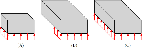
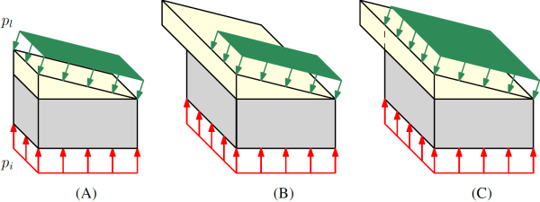
If the value is True, the interface pressure evolution computed in Metalub is applied to the lower edge of the strip. The edge is thus again pushed upwards. As mentioned before, it is important to take into account the out-of-plane thickness variation in the definition of this Traction2DElement. In fact, if the out-of-plane thickness of the strip increases, the area on which the interface pressure is applied increases, too. Although, the interface pressure was previously applied to this lower area, the computation does not automatically take into account its increase, which results in more important resultant nodal forces. Hence, the out-of-plane thickness variation of the strip is introduced in the definition of the Traction2DElement. The following figure illustrates what happens in the initial state (A) and when the elongation of the strip increases, if the previous condition is not taken into account (B) and if it is taken into account (C).
Moreover, in the second case (imposed interface pressure), an additional constraint is introduced to impose that this edge remains horizontal via the EqualityDofConstraintsSet (internally, this is possible by associating the degrees of freedom of several nodes to a same degree of freedom).
Edges of the lubricant
First, the horizontal displacement of the upper edge of the lubricant is always blocked due to the assumed non-deformation of the roll.
Second, two different conditions are possible for the remaining degrees of freedom of the left, upper and right edges of the lubricant. These conditions can be set separately for each of these edges, depending on the values of the variables bc_lubLeftEdge, bc_lubUpperEdge and bc_lubRightEdge.
If the variable corresponding to the upper edge is set equal to blocked, the vertical displacement is blocked in addition to the horizontal one. If the corresponding variable to the left or the right edge is set equal to blocked, the horizontal displacement of these edges is blocked.
If, however, one of these variables is set equal to pLcontrolled, the lubricant pressure evolution computed in Metalub is imposed to the corresponding edge. According to Carretta, this was at least necessary for the upper edge, the others being blocked, to reach a lubricant pressure in the cavity equal to the one computed with Metalub, although this pressure is already controlled by the imposed out-of-plane thickness evolution of the lubricant. More precisely, if all edges are blocked, the lubricant elongation condition does absolutely not lead to the same lubricant pressure evolution than in Metalub. If the lubricant pressure is imposed on the upper edge of the lubricant, the evolution is qualitatively similar but quantitatively different by a few percent (than the result in Metalub).

In the previous version, the out-of-plane thickness evolution of the lubricant was not introduced in the definition of the traction element, but the pressure was multiplied explicitly by the out-of-plane thickness. In this new version, it was included in the definition of the traction element by specially paying attention to the zone to which it is applied. To illustrate this subtlety, the following figure shows the scenario in which the lubricant pressure from Metalub is only applied to the upper edge of the lubricant (not on the left and right edges of the lubricant). Case (A) shows the initial state. Case (B) shows the state in which the elongation of the strip is not taken into account. Finally, case (C) shows what is currently implemented in the asperity crushing model, i.e. that the elongation of the strip (not of the lubricant!) is introduced in the Traction2DElement, which is applied to the upper edge of the lubricant.
Contact interaction
As explained earlier, the contact tool is shifted by a distance $h_{p}$ downwards from the upper edge of the lubricant to create small lubricant pipes. These pipes were created to model the transition from the hydrodynamic regime, i.e. no contact between the strip and the roll, to the mixed lubrication regime, i.e. the contact pressure is partially supported by the strip, partially by the lubricant.
Hence, when the contact tool enters into contact with the upper edge of the strip, the relative contact area between the roll and the strip increases. Simultaneously, the lubricant pressure increases in the whole lubricant domain since all lubricant elements are connected due to the small elements in the pipes. It was hoped to observe a later separation between the contact tool and the upper edge of the strip due to the increasing lubricant pressure (hydrodynamic effect), at the time Carretta developped these tests.
Different contact tool laws (based on the penality method) can be defined depending on the value of the variable contLaw (see Contact materials):
FLess:FrictionlessContactMaterialCoulomb:CoulombContactMaterialStick:StickingVariablePenaltyContactMaterial
In the definition of the contact interaction, it is important to mention the options AIC_ONCEPERSTEP and AICBS_INTERNAL. While the first option leads to an update of the nodal contact area at the slave nodes at each time step (see section about Extractors below), the second option renders it possible to take into account the contact between the upper edge of the strip and the contact tool although this edge is located inside of the volume (between the lubricant and the strip) instead of the outside of the volume.

ALE
The ALE method is used to prevent important mesh distortions of the lubricant. It is activated all nAle time steps, if ale is true. As explained earlier, the rezoners were defined in the files geoTriang1.py, geoTriang2.py and geoSpline.py.
Either Godunov's method or the finite volume linear reconstruction method (see Formalisme A.L.E.) can be used for the convection step with sub-stepping depending on whether conv is equal to godunov or benson. Only the pressure is convected. More precisely, to compute the pressure, Metafor computes a pressure increment at each time step based on the bulk modulus and the volume variation of the lubricant elements. To compute the pressure at the following time step it is therefore necessary to convect the pressure.
According to Carretta, the velocities and accelerations were not convected because they made the convergence more difficult/impossible.

Execution modes
Different execution modes of the general asperity crushing simulation in the file aspCrush.py are possible by setting the following variables to True or False:
postProOn: if True, the extractors are defined and added to the values manager. Hence, .ascii data files are created during the simulation and their values are written to these files for each time step. In consequence, the size of the files can become relatively important. For this reason, it is possible to setpostProOnto False and thus, to not create the files during the simulation. It is, however, possible to create the files afterwards based on the FAC files (at reduced sampling frequency obviously, since less FAC files are usually written than there are time steps) by executing thepostPro()function of the test case files or theaspCrush.pyfile.
batteryOn: if True, only some time steps are computed in order to reduce the computation time to a minimum for the battery test cases. In this case, the previous variablepostProOnhas no importance since the extractors should be tested in any case, i.e. everything happens as ifpostProOnwas equal to True. IfbatteryOnis set equal to False, an entire asperity crushing simulation is computed. The type of simulation depends on the variablebc_pLoweras explained earlier. If this variable is False, the simulation proceeds until the imposed displacement is reached. If it is True, the interface pressure is applied until reaching its last value imported from Metalub.
plotCurves: if True, some data curves are plotted. In particular, the interface and lubricant pressure evolutions along the roll bite and the out-of-plane thickness evolutions of the lubricant and the strip along the roll bite. This option can only be activated, if the previous variablepostProOnis True.
Extractors
The different extractors were defined in the file aspExtr.py, as mentioned above. They are used to create the following files and the corresponding values, which are used by Metalub in the coupling procedure:
xFEM.ascii: position along the roll biteaFEM.ascii: corresponding relative contact areahtFEM.ascii: corresponding distance between updated mean linesplFEM.ascii: corresponding lubricant pressurepaFEM.ascii: corresponding asperity contact pressure
Position along the roll bite
The position along the roll bite can be computed easily by inverting the previous space-to-time relation (see Boundary conditions hereabove), i.e.
\begin{equation} x = v (t - t_{0}) + x_{0} \end{equation}
Relative contact area
The relative contact area $A$ is equal to the ratio of the real and the apparent contact areas, i.e. $A = A_{r}/A_{a}$. In Metafor, the real contact area $A_{r}$ can be approximated by the sum of the nodal contact areas $a_{i}$ of the nodes $i$ in contact with the tool.
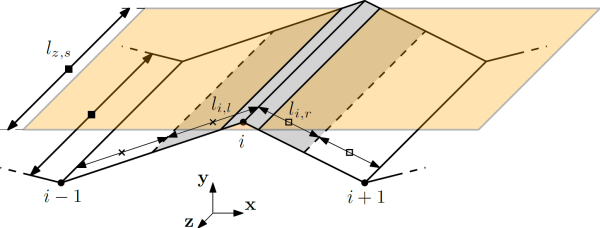
In fact, to compute the contact area it is necessary to estimate the nodal areas $a_{i}$, i.e. the area of contact associated to a node $i$. A rough approximation, which becomes more and more precise when the element size decreases, is to compute the nodal contact area as the sum of the half-lengths of the incident edges multiplied by the out-of-plane thickness. More precisely, the following figure shows the contact tool in orange that enters into contact with the strip at the node $i$. Hence, the nodal contact area is given by the following equation:
\begin{equation} a_{i} = (l_{i,l} + l_{i,r}) l_{z,s} \end{equation}
As explained before (section about the “Contact interaction”), it is currently not possible to take into account the evolution of the out-of-plane thickness of the strip in the contact interaction. In consequence, Metafor rather computes the nodal contact area as follows ($l_{z,s} = 1.0$):
\begin{equation} a_{i} = l_{i,l} + l_{i,r} \end{equation}
Since the out-of-plane thickness of the strip was used in the definition of the nodal contact areas, the apparent contact area $A_{a}$ is equal to the length of the contact tool $l_{c}$ multiplied by the unit thickness 1.0. Hence, the relative contact area $A$ is given by
\begin{equation} A = \frac{\sum_{i} c_{i} a_{i}}{l_{c}} \qquad \text{where} \qquad c_{i} = \begin{cases} 1, \text{ if in contact} \\ 0, \text{ otherwise} \end{cases} \end{equation}
Previously mentioning the option AIC_ONCEPERSTEP in the definition of the contact interaction ensures that the values $a_{i}$ are updated after each time step.
Distance between updated mean lines
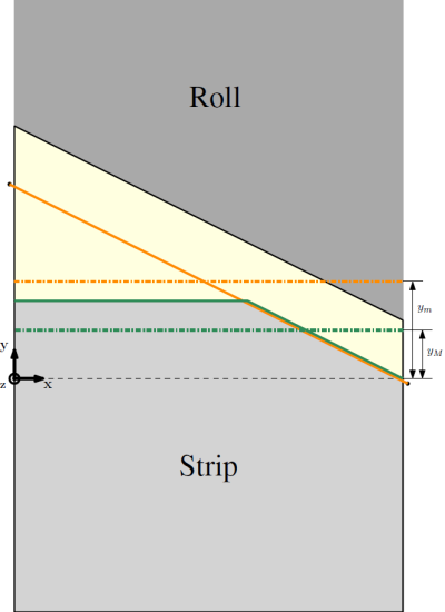
The distance between updated mean lines is computed as follows, since the pipe thickness is very small:
\begin{equation} h_{t} = y_{m} - y_{M} \end{equation}
where
- $y_{m}$ is the vertical position of the mean line of the contact tool, i.e. the roll;
- $y_{M}$ is the vertical position of the updated mean line of the strip profile.
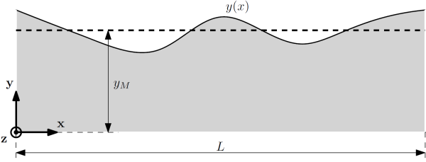
While $y_{m}$ does not change during the computation since the tool is rigid, the mean line of the strip profile has to be updated based on its definition:
\begin{equation} y_{M} = \frac{1}{L} \int_{0}^{L} y(x) \; \text{d}x \end{equation}
Moreover, a relaxation is used to update the difference between mean lines to improve the convergence, i.e.
\begin{equation} h_{t}(x) = (1 - w) \; h_{t, \text{Metalub}}(x) + w \; h_{t, \text{Metafor}}(x) \end{equation}
where $w$ is a relaxation factor currently equal to 0.1. The $x$ in the previous equation represent the position in the roll bite in Metalub, i.e. not the $x$-coordinate in Metafor.
Lubricant pressure applied to the strip
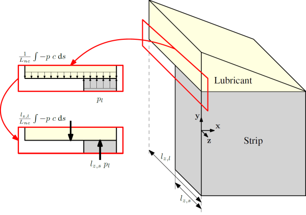
The lubricant pressure is determined by first computing the average pressure in the lubricant domain by the following integral along the upper edge of the lubricant: \begin{equation} \frac{1}{L_{nc}} \int -p \; c \; \text{d}s = \frac{1}{L_{nc}} \int -p(x) \; c \; \sqrt{1 + \left(\frac{\partial y}{\partial x}\right)^{2}} \; \text{d}x \end{equation}
where
- $p(x)$ is the pressure at the nodes of the upper edge of the lubricant. The minus sign was introduced since the pressure for a compressive state is negative in Metafor but positive in Metalub and since the pressure value is extracted from Metafor to use it in Metalub;
- $c$ is a variable that is equal to 0, if the corresponding node on the upper edge of the strip to the node at which the pressure is extracted on the upper edge of the lubricant is in contact with the contact tool. This correspondence is only possible due to the particular structure of the mesh. If there is no contact at the corresponding node, $c$ is equal to 1.
- $\text{d}s$ is the infinitesimal arc length element of the upper edge of the lubricant. The position of the upper edge is given by the function $y(x)$ in the Cartesian coordinate system. Hence, the integral can be written as an integral along $x$.
- $L_{nc}$ is the length of the upper edge of the lubricant for which the corresponding nodes on the upper edge of the strip are not in contact (nc) with the contact tool, i.e.
\begin{equation} L_{nc} = \int c \; \text{d}s \end{equation}
It is important to notice that the previous average pressure in the lubricant domain is not necessarily equal to the lubricant pressure applied to the strip. In fact, the areas with respect to which these pressures are calculated can be different. More precisely, the lubricant area is the lubricant elongation $l_{z,l}$ times the width along $\mathbf{x}$ while the strip area is the strip elongation $l_{z,s}$ times the width along $\mathbf{x}$ (see figure below). If $l_{z,l}$ and $l_{z,s}$ are different, the average pressure in the lubricant domain is thus not equal to the lubricant pressure applied to the strip. Both values are, however, related since the equilibrium of forces is computed by the finite element method: \begin{equation} \frac{l_{z,l}}{L_{nc}} \int -p \; c \; \text{d}s = l_{z,s} \; p_{l} \end{equation}
Isolating the lubricant pressure applied to the strip $p_{l}$ eventually leads to the formula which is used to compute its value:
\begin{equation} p_{l} = \frac{l_{z,l}}{l_{z,s}} \frac{1}{L_{nc}} \int -p \; c \; \text{d}s = \frac{l_{z,l}}{l_{z,s}} \frac{1}{L_{nc}} \int -p(x) \; c \; \sqrt{1 + \left(\frac{\partial y}{\partial x}\right)^{2}} \; \text{d}x \end{equation}
Asperity contact pressure
The asperity contact pressure $p_{a}$ is finally determined based on the sharing law (see Metalub reference document for more details): \begin{equation} p_{i} = A p_{a} + (1 - A) p_{l} \end{equation} where $p_{i}$, $A$ and $p_{l}$ are the interface pressure, the relative contact area and the lubricant pressure. The interface pressure was imposed on the lower edge of the strip. It can thus either be extracted of the Metalub result file or of the simulation by an extractor. This later case was chosen to double-check the results. Hence, the sum of the forces on the lower edge of the strip is divided by the width along $\mathbf{x}$ and the out-of-plane thickness of the strip portion to obtain the interface pressure.
Since the relative contact area and the lubricant pressure are known from the previous extractors, the asperity contact pressure is finally given by the following formula (based on the previous one): \begin{equation} p_{a} = \frac{p_{i} - (1 - A)p_{l}}{A} \end{equation}
Changes of results of the battery test cases
Besides renaming the test cases, changes of results of the battery test cases are due to the following reasons:
- Wrong computation of the mean line of the contact tool in the scenario with the two triangular half asperities (see the section related to the “Two triangular half asperities” for more details);
- It was thought that the out-of-plane thickness evolution of the strip (introduced in the contact interaction) was taken into account to compute the nodal areas of the slave nodes. But it was not. Hence, the computation of the relative contact area included the out-of-plane thickness in the denominator, though it should not be included.
Added [a] / deleted [d] / modified [m] / renamed [r] general files/folders
[m] CMakeLists.txt

[m] aspCrushing/tools/python/rollingAsp.py
[r] aspCrushing/tools/python/aspCrush.py

[m] aspCrushing/tools/python/aspExtractors.py
[r] aspCrushing/tools/python/aspExtr.py

[d] aspCrushing/tools/python/bCondPb.py

[m] aspCrushing/tools/python/evolutionFunction.py
[m] aspCrushing/tools/python/geoSpline.py

[m] aspCrushing/tools/python/geoTriang.py
[r] aspCrushing/tools/python/geoTriangle1.py

[m] aspCrushing/tools/python/geoTwoAsp.py
[r] aspCrushing/tools/python/geoTriangle2.py

[m] aspCrushing/tools/python/Vector.py

[d] aspCrushing/tests/twoDhalf/bCond
[r] aspCrushing/tests/twoDhalf/bc
[d] aspCrushing/tests/twoDhalf/bCond/res_bc_ht.ascii
[r] aspCrushing/tests/twoDhalf/bc/res_bc_ht.ascii
[d] aspCrushing/tests/twoDhalf/bCond/res_bc_lxx.ascii
[r] aspCrushing/tests/twoDhalf/bc/res_bc_lx.ascii
[d] aspCrushing/tests/twoDhalf/bCond/res_bc_lxx_lub.ascii
[r] aspCrushing/tests/twoDhalf/bc/res_bc_lx_lub.ascii
[d] aspCrushing/tests/twoDhalf/bCond/res_bc_p.ascii
[r] aspCrushing/tests/twoDhalf/bc/res_bc_p.ascii
[d] aspCrushing/tests/twoDhalf/bCond/res_bc_pb_rey.ascii
[r] aspCrushing/tests/twoDhalf/bc/res_bc_pl.ascii
[d] aspCrushing/tests/twoDhalf/bCond/res_bc_p.ascii
[r] aspCrushing/tests/twoDhalf/bc/res_bc_pi.ascii
Added [a] / deleted [d] / modified [m] / renamed [r] test cases
[m] aspCrushing/tests/twoDhalf/reelDry.py
[r] aspCrushing/tests/twoDhalf/splineDry.py
[m] aspCrushing/tests/twoDhalf/reelDry.tsc
[r] aspCrushing/tests/twoDhalf/splineDry.tsc

[m] aspCrushing/tests/twoDhalf/reelLub.py
[r] aspCrushing/tests/twoDhalf/splineLub.py
[m] aspCrushing/tests/twoDhalf/reelLub.tsc
[r] aspCrushing/tests/twoDhalf/splineLub.tsc

[m] aspCrushing/tests/twoDhalf/triang1Dry.py
[r] aspCrushing/tests/twoDhalf/triangle1Dry.py
[m] aspCrushing/tests/twoDhalf/triang1Dry.tsc
[r] aspCrushing/tests/twoDhalf/triangle1Dry.tsc

[m] aspCrushing/tests/twoDhalf/triang1Lub.py
[r] aspCrushing/tests/twoDhalf/triangle1Lub.py
[m] aspCrushing/tests/twoDhalf/triang1Lub.tsc
[r] aspCrushing/tests/twoDhalf/triangle1Lub.tsc

[m] aspCrushing/tests/twoDhalf/triang2Dry.py
[r] aspCrushing/tests/twoDhalf/triangle2Dry.py
[m] aspCrushing/tests/twoDhalf/triang2Dry.tsc
[r] aspCrushing/tests/twoDhalf/triangle2Dry.tsc

[m] aspCrushing/tests/twoDhalf/triang2Lub.py
[r] aspCrushing/tests/twoDhalf/triangle2Lub.py
[m] aspCrushing/tests/twoDhalf/triang2Lub.tsc
[r] aspCrushing/tests/twoDhalf/triangle2Lub.tsc
— Dominik Boemer 2017/12/20 11:30
