How to run an existing test?

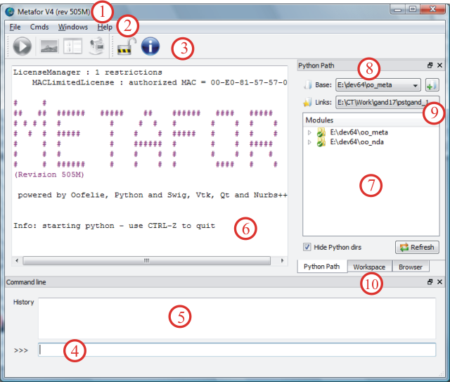
Double-click the “Run Metafor” icon on your desktop. The GUI is displayed:

1. The title bar. It contains the version number of your Metafor executable.
2. The menu bar. It is useful for managing interface options (File menu / GUI Options) and 3D active display windows (Windows menu).
3. The toolbar. It gathers the most commonly used commands, such as the meta() button (blue PLAY button) which initiates a Metafor calculation.
4. The python command line: it allows the user to enter Metafor commands by hand or to use Metafor as a simple python interpreter.
5. The history command window: quick access to copy/paste older commands. A contextual menu allows the user to manage the history.
6. The output python window, which displays the text output of the program.
7. The “Python PATH”, which lists all available python modules that can be imported.
8. The “base” folder, which is the current folder at startup. It can be changed to a new folder which will be added to the “Python PATH”. This is very useful to run a test located on a non-standard path (e.g. on another hard disk partition).
9. The links. This widget gathers the last loaded modules for faster access.
10. The “workspace”. This is the place where the results of a calculation are written to disk.

A test case of Metafor corresponds to usually one python module.

Therefore, the first step usually consists in loading this module into memory. This operation tells the program that you wish to work with this file, whether for running an integration or viewing results.

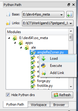
To load a module with the GUI, just find it in the “Python PATH” tree. then right-click on it and choose “Load”.

Alternatively, use the command

load('apps.ale.angleReZoner') 

in the python command line. This command loads the module angleReZoner.py, located in c:\Program Files\Metafor\apps\ale.

Metafor “imports” the module and keeps a pointer to it for subsequent commands. The interface on the right switches from “Python PATH” view to “Workspace” view. In this view, a working directory (in which the results of the simulation will be stored) can be chosen. By default, its name is workspace/module_name. If it already exists, this directory is selected by the interface. If not, it will be created before the beginning of the time integration.

If the module to be loaded is not in the “Python PATH”, a rebase must be performed. To do so, the directory which contains the test case is chosen using the button on the “Base” line of the “Python Path” tab. Doing so, this directory is added to the “Python path”. It is equivalent to starting Metafor from this directory.

Click on the blue “PLAY” button in the toolbar. You can also type the command:

meta()

This command calls the function getMetafor() defined in the module previously loaded, and starts the time integration. If no working directory was explicitly selected, the default name (workspace/test_name) is used. If this directory already contains older results, those files will be first deleted (after user's approval).

Then, the time integration procedure opens a 3D graphics window, which will be continuously refreshed during computation displaying the current results. The display options can be modified using the “Config” button of this window.

It is possible to close the display windows, and reopen them using the “Windows” menu.

When the time integration finishes, you MUST restart Metafor to run another test !

To load previously-computed results, the corresponding module must be loaded first, as was done before starting the time integration. Then, if the workspace used is the default one, Metafor automatically sets its working directory to it. Otherwise, it must be changed manually, using the workspace window.

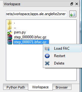
Once the right folder is selected, simply locate the “FAC” files (extension .bfac.gz), choose one and load it with the context menu (“Load Fac”). The results are displayed in a graphical window.

To load other results, repeat the operation with other FAC files. The display window is updated automatically.

For various reasons (power cut, abrupt closure of Metafor…), a simulation may have ended earlier than expected. However, it can be restarted from an intermediate FAC, usually the last one that was written before the breakdown (therefore, several saving points should be planned before running long computations).

This is rather straightforward :

• load the right module
• if you do not use the default workspace, set the right working directory.
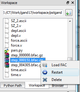
• choose the last FAC and restart it with the context menu

The integration starts again from the selected FAC file.

<html> <center> <embed width=“320” height=“240” src=“http://metafor.ltas.ulg.ac.be/oldsite/flv/flvplayer.swf?file=http://metafor.ltas.ulg.ac.be/oldsite/flv/tuto.flv” quality=“high” type=“application/x-shockwave-flash” /> </center> </html>

To show results in a pleasant way, an “.avi” file, showing the integration over time, can be created.

• First, increase the number of times that results will be saved to disk. (command setNextTime of TimeStepManager, see Managing Time Steps)
• Run the test.
• Load the last FAC file. Set up the scale of displayed scalar values according to their final value. Do the same for vectors, if needed. Then save the graphical options (“Save” button).
• Restart Metafor, load your module. Click on makeAnimation() in the toolbar. The first time step is displayed, and other display options (such as zoom, camera…) can be adjusted.
• Press [ENTER] in the python command line. Metafor will then load all FAC files and successively perform screenshots. These are saved in the workspace, format bmp.
• Finally, use a software like AVIMaker to create the video from screenshots. Ideally, you should use a “lossless codec”, for example Microsoft Video in highest quality.

Should you need to run Metafor in command line, open a command line (cmd.exe, or a Unix shell). Then :

• metafor -help : display help
• metafor -nogui : start Metafor without the GUI
• metafor -nogui -run apps.qs.cont2 : run load/meta on apps/qs/cont2.py
• metafor -nogui myscript.py : execute commands written in myscript.py.

In interactive mode, after metafor -nogui, we find ourselves in a python interpreter where some specific Metafor modules were loaded. To exit Metafor in “text” mode, on Windows, use CTRL-BREAK (a little rough, but that works), or CTRL-Z then Enter on Windows, or finally CTRL-D on Unix.

To run a test :

load('apps.qs.cont2')
meta()

To execute a script (such as postprocessing) :

execfile('myscript.py')

To exit the command line, use CTRL-Z on Windows, CTRL-D on Linux/Unix.

Now, you know how to use the GUI, run a test and display results. We will then learn how to build your own data set :

⇒ Python in a nutshell